
Target audience: Intermediate
Estimated reading time: 5'
Ever hoped for numpy to offer automatic differentiation and run math computations on a GPU? You might find DeepMind's JAX to be the solution.
In this piece, we'll delve into JAX's automatic differentiation capabilities and assess how its just-in-time execution compares to numpy.

Table of contents
Notes:
- Library versions: python 3.11, JAX 0.4.18, Jax-metal 0.0.4 (Mac M1/M2), NumPy 1.26.0, matplotlib 3.8.0
- To enhance the readability of the algorithm implementations, we have omitted non-essential code elements like error checking, comments, exceptions, validation of class and method arguments, scoping qualifiers, and import statements.
- The performance evaluation Performance: JAX vs NumPy relies on AWS m4.2xlarge EC2 instance for CPU and p3.2xlarge instance equipped with 8 virtual cores, 64GB of memory, and an Nvidia V100 GPU.
- JAX provides developers with a profiler to generate traces that can be visualized using the Perfetto visualizer.
Introduction
As a quick recall, NumPy stands as a Python library for numerical and scientific computation. It equips data scientists and engineers with capabilities for working with multidimensional arrays, performing speedy array operations, and handling fundamental tasks in linear algebra and statistics [ref 1].
JAX [ref 2] is a numerical computing and machine learning library in Python, developed by DeepMind, that builds upon the foundation of NumPy. JAX offers:
- Composable function transformations.
- Auto-vectorization of data batches, enabling parallel processing.
- First and second-order automatic differentiation for various numerical functions.
- Just-in-time compilation for GPU execution [ref 3].
Components
- AutoGrad: Upgraded to improve performance of automatic differentiation.
- Accelerated Linear Algebra (XLA): JAX uses XLA to compile and run your NumPy code on accelerators.
- Just-in-time compilation (JIT): Running on XLA
- Perfetto: Visualization of profiler trace data.
Installation
Here is an overview of basic steps for installing JAX. It is advisable to consult the installation guide as each environment has specific requirements [ref 4].
CPU (MacOS, Linux)
- pip install --upgrade "jax[cpu]"
GPU (Linux/CUDA)
- nvcc --version # -> ve to be used in the
- pip install --upgrade "jax[cuda12_pip]" -f https://storage.googleapis.com/jax-releases/jax_cuda_releases.html
GPU (MacOS/mps)
- python3 -m venv ~/jax-metal
- source ~/jax-metal/bin/activate
- python -m pip install jax-metal
- pip install ml_dtypes==0.2.0
Conda
- conda install jax -c conda-forge
Automatic differentiation
Overview
Automatic differentiation is a tool that facilitates the automatic calculation of derivatives for a specified mathematical function [ref 5].
This technique efficiently determines precise derivatives by retaining details during the forward pass, which are then utilized during the backward pass. Essentially,
- It interprets a code that calculates a function and leverages it to compute the function's derivative.
- It crafts a software approach to efficiently determine the derivatives, bypassing the necessity for a closed-form solution.
This article focuses on the Forward Mode Automatic Differentiation, which consists of replacing each primitive operation in the original program by its differential analogue.
To illustrate the concept, let consider the function \[f(x,y,z)=2x^{2}-3xy+z \] Let's build its forward computation graph:

fig 1. Simplified forward computation graph
Notes:
- This computation graph does not include data type conversion (Python values to JAX or NumPy arrays).
- The limitation of the forward mode is that the gradient is computed by re-executing the program all over again. The solution is to stored the derivatives to be chained and computed during a backward path: Reverse Model Automatic Differentiation.
Single variable function
Let's implement a class, JaxDifferentiation that wraps the computation of first, second, ... derivatives of a function with a single variable. \[func: \mathbb{R} \rightarrow \mathbb{R}\].The derivative of various orders are computed in the constructor. The method __call__ return the list [f, f', f", ..].
class JaxDifferentiation(object):
    """
        Create a set of derivatives of first, second, ... order_derivative order
        :param func Differentiable function
        :param Order of derivatibes
    """
    def __init__(self, func: Callable[[float], float], order_derivative: int):
        assert order_derivative < 5, f'Order derivatives {order_derivative} should be [0, 4]'

        # Build list of derivative f, f', f", ....
        self.derivatives: List[Callable[[float], float]] = [func]
        temp = func
        if order_derivative > 0:
            for order in range(order_derivative):
                # Compute the single variable next order derivative
                temp = jnp.grad(temp)
                self.derivatives.append(temp)
    def __call__(self, x: float) -> List[float]:
        """ Compute derivatives of all orders for value x"""
        return [derivative(x) for derivative in self.derivatives]
Let's compute the derivative of the following function.\[\\ f(x)=2.x^{4}+x^{3} \\ \\ \frac{\mathrm{d} f}{\mathrm{d} x}=8.x^{3}+3.x^{2} \\ \\ \frac{d^{2}f}{dx^{2}}=24.x^{2}+6.x\]. The first and second derivatives are provided for evaluation purpose (Oracle).
# Function definitiondef func1(x: float) -> float:
return 2.0*x**4 + x**3
# First order derivative
def dfunc1(x: float) -> float:
   return 8.0*x**3 + 3*x**2
# Second order derivativedef ddfunc1(x: float) -> float:
   return 24.0*x**2 + 6.0*x

funcs1 = [func1, dfunc1, ddfunc1]
jax_differentiation = JaxDifferentiation(func1, len(funcs1))
compared = [f'{oracle}, {jax_value}, {oracle-jax_value}'
for oracle, jax_value in zip([func(y) for func in funcs1], jax_differentiation(2.0))]
print(compared)
Output
Oracle, Jax, Difference
40.0, 40.0, 0.0
76.0, 76.0, 0.0
108.0, 108.0, 0.0
Multi-variable function
The next step is to evaluate the computation of partial derivative of a multi-variable function f(x,y,...)\[J=[\frac{\partial f}{\partial x_{1}}, \frac{\partial f}{\partial x_{2}}, ..., \frac{\partial f}{\partial x_{n}}]\]
Let's consider the following function for which the first order partial derivative (Jacobian vector) is provided. \[\\ f(x,y,z)=2x^{2}-3xy+z \\ \\ \frac{\partial f}{\partial x} = (4x -3y) ; \frac{\partial f}{\partial y} = -3x ; \frac{\partial f}{\partial z} = 1.0\]
# Function definitiondef func2(x: List[float]) -> float:
return 2.0*x[0]*x[0] - 3.0*x[0]*x[1] + x[2]
# Partial derivative over xdef dfunc2_x(x: List[float]) -> float:
  return 4.0*x[0] - 3.0*x[1]
# Partial derivative over ydef dfunc2_y(x: List[float]) -> float:
  return -3.0*x[0]
# Partial derivative over zdef dfunc2_z(x: List[float]) -> float:
  return 1.0
Let's compare the output of the direct computation of the symbolic derivatives (Oracle) dfunc2_x, dfunc2_y and dfunc2_z with the partial derivatives computed by JAX.
We use the forward mode automatic differentiation function jacfwd to compute the gradient [ref 6].
# Invoke the Jacobian vector forward function dfunc2 = jnp.jacfwd(func2)
y = [2.0, -1.0, 6.0]
derivatives = dfunc2(y)
print(f'df/dx: {derivatives[0]}, {dfunc2_x(y)}\ndf/dy: {derivatives[1]}, {dfunc2_y(y)}\ndf/dz: {derivatives[2]}, {dfunc2_z(y)}'
)Oracle, Jax
df/dx: 11.0, 11.0
df/dy: -6.0, -6.0
df/dz; 1.0, 1.0
Note: The reverse mode automatic differentiation Jax method, jacrev would have produce the same result.
Performance: JAX vs NumPy
A significant drawback of the NumPy library is its absence of GPU support. The next objective is to measure the performance gains achieved by JAX, with and without its just-in-time compiler, on both CPU and GPU.
To facilitate this, we will establish a class named JaxNumpyData containing two functions: np_func, which utilizes NumPy, and jnp_func, its JAX counterpart. These functions will be applied to datasets of various sizes. The compare method will extract 20 subsets from the initial dataset by employing a basic fraction-based approach.
class JaxNumpyData(object): """ Initialize the numpy and Jax function to process data (arrays) :param np_function Numpy numerical function :param jnp_function Corresponding Jax numerical function """
def __init__(self,
np_func: Callable[[np.array], np.array],
jnp_func: Callable[[jnp.array], jnp.array]):
self.np_func = np_func
self.jnp_func = jnp_func
def compare(self, full_data_size: int, func_label: AnyStr): """ Compare the :param full_data_size Size of the original dataset used to extract sub-data set :param func_label Label used for performance results and plotting """ for index in range(1, 20):
fraction = 0.05 * index
data_size = int(full_data_size*fraction)
            # Execute on the full_data_size*fraction element using Numpy            x_0 = np.linspace(0.0, 100.0, data_size)
            result1 = self.map_numpy(x_0, f'numpy_{func_label}')
            # Execute on the full_data_size*fraction element using JAX and JAX-JIT
            x_1 = jnp.linspace(0.0, 100.0, data_size)
            result2 = self.map_jax(x_1, f'jax_{func_label}')
            result3 = self.map_jif(x_1, f'jif_{func_label}')
del x_0, x_1, result1, result2, result3
     """ Process numpy array, np_x through numpy function np_func """    @time_it
    def map_numpy(self, np_x: np.array, label: AnyStr) -> np.array:
        return self.np_func(np_x)
     """ Process Jax array, jnp_x through Jax function jnp_func """    @time_it
    def map_jax(self, jnp_x: jnp.array, label: AnyStr) -> jnp.array:
        return self.jnp_func(jnp_x)
     """ Process Jax array, jnp_x through Jax function jnp_func using JIT """    @time_it
    def map_jif(self, jnp_x: jnp.array, label: AnyStr) -> jnp.array:
        from jax import jit
        return jit(self.jnp_func)(jnp_x)
The method map_numpy (resp. map_jax and map_jit) applies the NumPy method np_func (resp. JAX method jnp_func) to the NumPy array np_array (resp. JAX array jnp_array).
CPU
In this first performance test, we measure the duration to compute \[f(x) = sinh(x)+cos(x)\] on 1,000,000,000 values using NumPy, JAX w/o just in time compiler.
def np_func1(x: np.array) -> np.array:
    return np.sinh(x) + np.cos(x)

def jnp_func1(x: jnp.array) -> jnp.array:
    return jnp.sinh(x) + jnp.cos(x)
The JAX produces a 7 fold performance improvement over NumPy. The just in time processor adds another 35% improvement.
def np_func2(x: np.array) -> np.array:return np.mean(x)def jnp_func2(x: jnp.array) -> jnp.array:return jnp.mean(x)
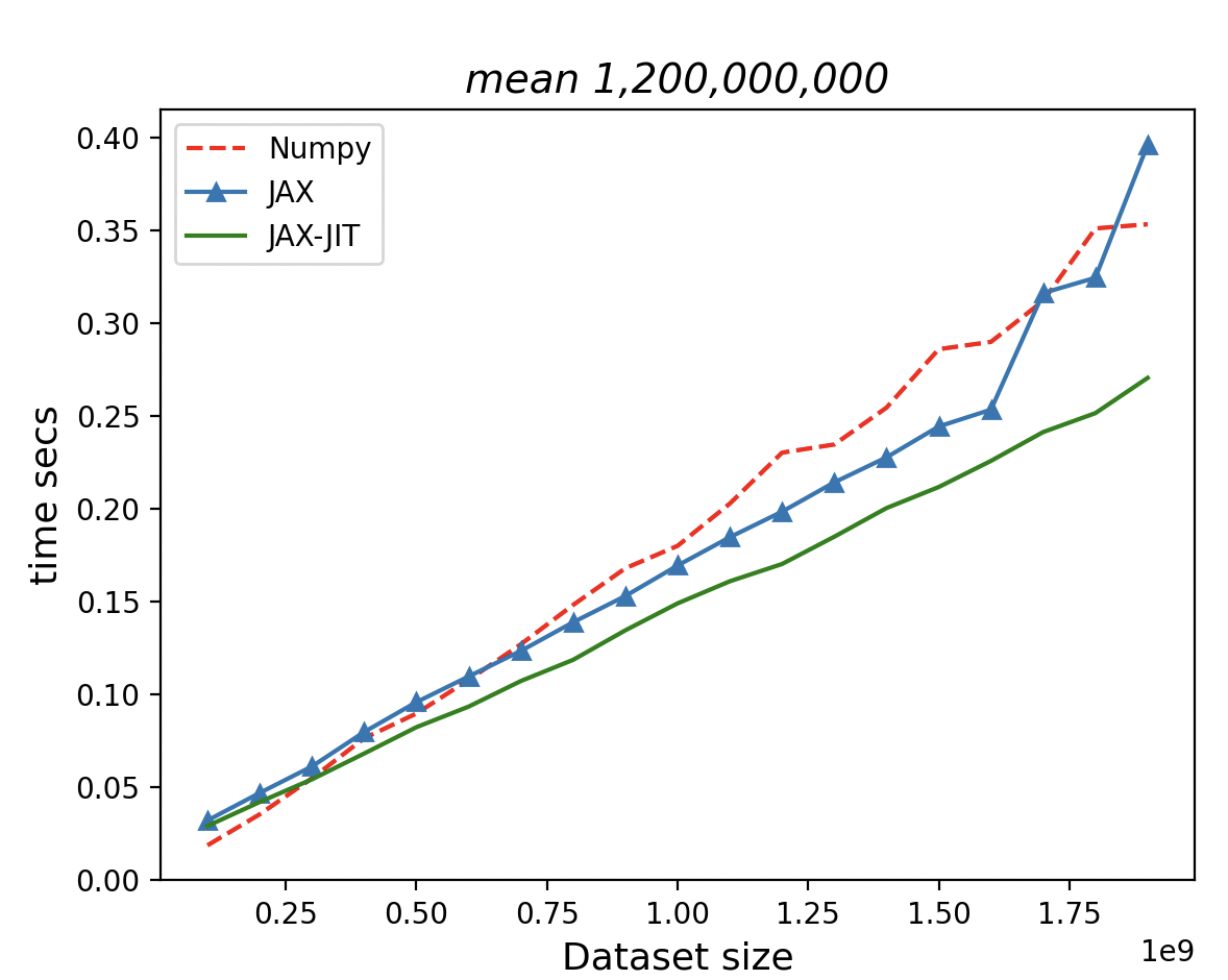
The just-in-time processor outperforms both NumPy and JAX native library on CPU.
GPU
For this last test, we execute the function \[f(x)=e^{-x} + cos(x))\] over 200,000,000 values on Nvidia V100 GPU.

As anticipated, NumPy is currently running on the CPU of the EC2 instance, which means it cannot match the performance of JAX running on the Nvidia processor.
Conclusion
In summary, JAX offers data scientists and machine learning engineers a high-performance GPU computing tool that significantly outperforms the NumPy library. Our exploration has only touched the surface of JAX's capabilities, and I encourage readers to delve deeper into features like Autobatching, Vectorization, Generalized convolutions, and its integration with PyTorch and TensorFlow.
Thank you for reading this article. For more information ...
References
[1] NumPy user guide
[4] Installing JAX
Appendix
We include the decorator used for timing the execution of the various functions, for reference.
timing_stats = {}
def time_it(func):
    """ Decorator for timing execution of methods """
    def wrapper(*args, **kwargs):
        start = time.time()
        func(*args, **kwargs)
        duration = '{:.3f}'.format(time.time() - start)
        key: AnyStr = args[2]
        print(f'{key}\t{duration} secs.')
        cur_list = timing_stats.get(key)
        if cur_list is None:
            cur_list = [time.time() - start]
        else:
            cur_list.append(time.time() - start)
        timing_stats[key] = cur_list
        return 0
    return wrapper
---------------------------
Patrick Nicolas has over 25 years of experience in software and data engineering, architecture design and end-to-end deployment and support with extensive knowledge in machine learning.
He has been director of data engineering at Aideo Technologies since 2017 and he is the author of "Scala for Machine Learning" Packt Publishing ISBN 978-1-78712-238-3
He has been director of data engineering at Aideo Technologies since 2017 and he is the author of "Scala for Machine Learning" Packt Publishing ISBN 978-1-78712-238-3


